Master Bayesian Analysis with Stan
Go from probability foundations to production Stan models under Scott Spencer — Columbia University professor and author of the course that top sports analytics teams recommend. Real sports data. Real inference. Real career impact.
Every student gets access to enterprise cloud virtual machines with Stan pre-configured, directly through the AthlyticZ Academy LMS.
The Skill That Separates Senior from Junior
Point estimates with no uncertainty
Stakeholders get a single number. No credible intervals, no honest communication of what the data actually says.
Full posterior distributions
Communicate uncertainty credibly with posteriors. Show stakeholders the range of plausible outcomes, not just one guess.
Black-box ML with no domain knowledge
Models that ignore what experts already know. Overfitting to noise in small datasets. No way to encode prior information.
Principled priors + evidence
Encode domain expertise as priors. Update beliefs with data. Get interpretable, regularized models that work with small samples.
Stuck at “I know the theory”
You read the textbook. You watched the lectures. But you can't write a Stan model, diagnose MCMC issues, or ship results.
Production Stan from day one
Code, compile, fit, diagnose. 28 Stan model files. Every concept becomes working code you can ship.

Scott Spencer
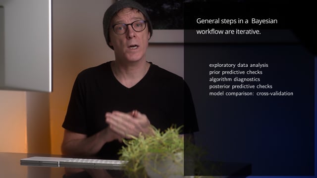
Scott Spencer teaches Bayesian statistics at Columbia University and has trained analysts across professional sports, pharma, and tech. His approach emphasizes building intuition through real data before touching any formula — then immediately translating that intuition into working Stan code.
His teaching method is distinctive: every concept is grounded in sports examples (Olympic sprints, basketball free throws, soccer expected goals) before being generalized to the broader statistical framework. Students leave with both deep understanding and production-ready skills.
From Probability to Production Stan
20 modules. 100+ lessons. 28 Stan model files. Click any module to see every lesson.
Develop deep intuition for uncertainty, probability, and distributions using sports examples. Master priors, likelihoods, and posteriors before touching Stan.
Intuition Before Formulas
Most Bayesian courses start with math and lose you by week two. Scott starts with Olympic sprints and basketball free throws — building intuition through data you can see and feel. By the time you write your first formula, you already understand what it means.
Write, compile, and fit your first Stan models. Understand MCMC engines (Metropolis-Hastings, HMC), grid approximation, and develop a consistent language for specifying models.
Stan Is the Gold Standard
Stan powers Bayesian inference at the FDA, Goldman Sachs, Google, and every major sports analytics department. Learning Stan is not optional for serious Bayesian work — it is the engine. This phase gives you the keys.
Code, compile, fit, and diagnose regression models in Stan. Extend to categorical predictors, multiple predictors, then generalized linear models — binomial, Poisson, and multinomial — with basketball and soccer data.
Basketball Free Throws. Soccer Goals. Olympic Sprints.
Every model in this phase is built on real sports data. You are not fitting toy examples — you are building the exact types of models that sports analytics teams use to evaluate players, predict outcomes, and make decisions worth millions.
Share strength across groups with partial pooling and reparameterization. Then build a complete expected goals (xG) model from scratch — the capstone that ties everything together.
Build a Soccer xG Model from Scratch in Stan
Not a tutorial walkthrough. A real expected goals model built iteratively — from simple Bernoulli to hierarchical with correlated predictors and reparameterization. This is the project you show employers. It demonstrates every skill in the course.
Trusted by Analytics Leaders

“Scott Spencer brings Bayesian modeling alive. He not only explains the math, but shows how to implement models in Stan that are clear, scalable, and ready for research or production.”
“AthlyticZ has completely transformed the learning approach to data science through the use of sports-based problems. The instructors are the best of the best.”
Enroll in Becoming a BayeZian I
Becoming a BayeZian I
- 20 modules, 100+ lessons
- 28 Stan model files included
- 14 real sports datasets
- Soccer xG capstone project
- Taught by Columbia professor Scott Spencer
- Quizzes & assessments throughout
- Certificate of completion
Stan pre-configured via AthlyticZ Academy LMS
Members pay $1,159 • Explore Membership
Get Both Bayesian Courses Together
Combine Becoming a BayeZian I + Becoming a BayeZian II into one bundle and save. Master foundations through advanced topics — survival models, multilevel GLMs, and diagnostics at scale.
Members Pay $1,159 for This Course
Plus unlimited cloud VM access, 10+ live sessions per month, the full replay library, and 20% off every course in the catalog.
Frequently Asked Questions
From Probability to
Production Stan
20 modules. 100+ lessons. 28 Stan model files. A soccer xG capstone you can show employers. Cloud virtual machines included.